


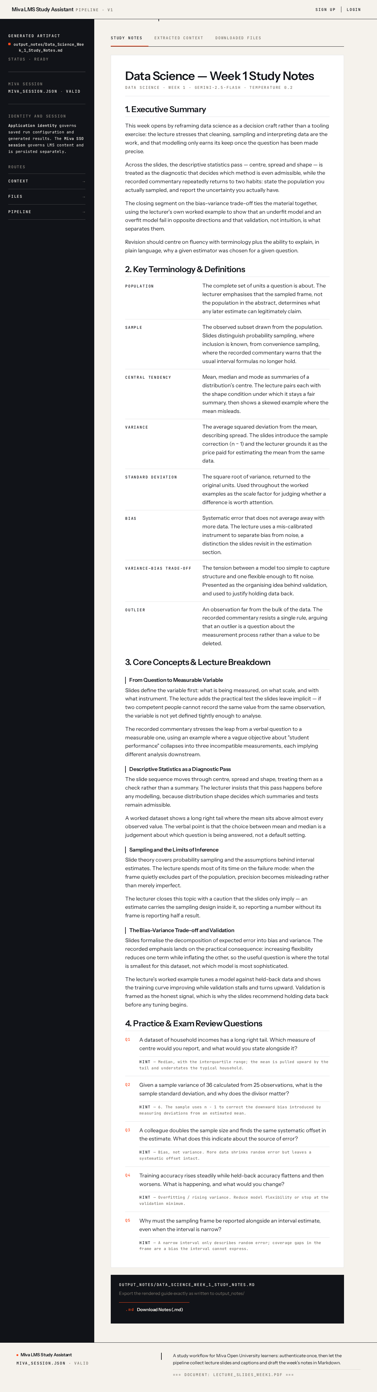
Data Science — Week 1 Study Notes
1. Executive Summary
This week opens by reframing data science as a decision craft rather than a tooling exercise: the lecture stresses that cleaning, sampling and interpreting data are the work, and that modelling only earns its keep once the question has been made precise.
Across the slides, the descriptive statistics pass — centre, spread and shape — is treated as the diagnostic that decides which method is even admissible, while the recorded commentary repeatedly returns to two habits: state the population you actually sampled, and report the uncertainty you actually have.
The closing segment on the bias–variance trade-off ties the material together, using the lecturer’s own worked example to show that an underfit model and an overfit model fail in opposite directions and that validation, not intuition, is what separates them.
Revision should centre on fluency with terminology plus the ability to explain, in plain language, why a given estimator was chosen for a given question.
2. Key Terminology & Definitions
- PopulationThe complete set of units a question is about. The lecturer emphasises that the sampled frame, not the population in the abstract, determines what any later estimate can legitimately claim.
- SampleThe observed subset drawn from the population. Slides distinguish probability sampling, where inclusion is known, from convenience sampling, where the recorded commentary warns that the usual interval formulas no longer hold.
- Central TendencyMean, median and mode as summaries of a distribution’s centre. The lecture pairs each with the shape condition under which it stays a fair summary, then shows a skewed example where the mean misleads.
- VarianceThe average squared deviation from the mean, describing spread. The slides introduce the sample correction (n − 1) and the lecturer grounds it as the price paid for estimating the mean from the same data.
- Standard DeviationThe square root of variance, returned to the original units. Used throughout the worked examples as the scale factor for judging whether a difference is worth attention.
- BiasSystematic error that does not average away with more data. The lecture uses a mis-calibrated instrument to separate bias from noise, a distinction the slides revisit in the estimation section.
- Variance–Bias Trade-offThe tension between a model too simple to capture structure and one flexible enough to fit noise. Presented as the organising idea behind validation, and used to justify holding data back.
- OutlierAn observation far from the bulk of the data. The recorded commentary resists a single rule, arguing that an outlier is a question about the measurement process rather than a value to be deleted.
3. Core Concepts & Lecture Breakdown
From Question to Measurable Variable
Slides define the variable first: what is being measured, on what scale, and with what instrument. The lecture adds the practical test the slides leave implicit — if two competent people cannot record the same value from the same observation, the variable is not yet defined tightly enough to analyse.
The recorded commentary stresses the leap from a verbal question to a measurable one, using an example where a vague objective about "student performance" collapses into three incompatible measurements, each implying different analysis downstream.
Descriptive Statistics as a Diagnostic Pass
The slide sequence moves through centre, spread and shape, treating them as a check rather than a summary. The lecturer insists that this pass happens before any modelling, because distribution shape decides which summaries and tests remain admissible.
A worked dataset shows a long right tail where the mean sits above almost every observed value. The verbal point is that the choice between mean and median is a judgement about which question is being answered, not a default setting.
Sampling and the Limits of Inference
Slide theory covers probability sampling and the assumptions behind interval estimates. The lecture spends most of its time on the failure mode: when the frame quietly excludes part of the population, precision becomes misleading rather than merely imperfect.
The lecturer closes this topic with a caution that the slides only imply — an estimate carries the sampling design inside it, so reporting a number without its frame is reporting half a result.
The Bias–Variance Trade-off and Validation
Slides formalise the decomposition of expected error into bias and variance. The recorded emphasis lands on the practical consequence: increasing flexibility reduces one term while inflating the other, so the useful question is where the total is smallest for this dataset, not which model is most sophisticated.
The lecture’s worked example tunes a model against held-back data and shows the training curve improving while validation stalls and turns upward. Validation is framed as the honest signal, which is why the slides recommend holding data back before any tuning begins.
4. Practice & Exam Review Questions
A dataset of household incomes has a long right tail. Which measure of centre would you report, and what would you state alongside it?
Hint — Median, with the interquartile range; the mean is pulled upward by the tail and understates the typical household.
Given a sample variance of 36 calculated from 25 observations, what is the sample standard deviation, and why does the divisor matter?
Hint — 6. The sample uses n − 1 to correct the downward bias introduced by measuring deviations from an estimated mean.
A colleague doubles the sample size and finds the same systematic offset in the estimate. What does this indicate about the source of error?
Hint — Bias, not variance. More data shrinks random error but leaves a systematic offset intact.
Training accuracy rises steadily while held-back accuracy flattens and then worsens. What is happening, and what would you change?
Hint — Overfitting / rising variance. Reduce model flexibility or stop at the validation minimum.
Why must the sampling frame be reported alongside an interval estimate, even when the interval is narrow?
Hint — A narrow interval only describes random error; coverage gaps in the frame are a bias the interval cannot express.
No comments yet. Be the first!